The Scientist and Engineer's Guide to
Digital Signal Processing
By Steven W. Smith, Ph.D.

• Home
• The Book by Chapters
• About the Book
  • Copyright and permissible use
  • What is DSP?
  • 8 good reasons for learning DSP
  • Comments by reviewers
  • Errata
  • Free Software and Teaching Aids
  • Differences Between Editions
• Steven W. Smith
• Blog
• Contact

The mean, indicated by μ (a lower case Greek mu), is the statistician's jargon for the average value of a signal. It is found just as you would expect: add all of the samples together, and divide by N. It looks like this in mathematical form:

In words, sum the values in the signal, x_i, by letting the index, i, run from 0 to N-1. Then finish the calculation by dividing the sum by N. This is identical to the equation: μ =(x₀ + x₁ + x₂ + ... + x_N-1)/N. If you are not already familiar with Σ (upper case Greek sigma) being used to indicate summation, study these equations carefully, and compare them with the computer program in Table 2-1. Summations of this type are abundant in DSP, and you need to understand this notation fully. In electronics, the mean is commonly called the DC (direct current) value. Likewise, AC (alternating current) refers to how the signal fluctuates around the mean value. If the signal is a simple repetitive waveform, such as a sine or square wave, its excursions can be described by its peak-to-peak amplitude. Unfortunately, most acquired signals do not show a well defined peak-to-peak value, but have a random nature, such as the signals in Fig. 2-1. A more generalized method must be used in these cases, called the standard deviation, denoted by σ (a lower case Greek sigma).

As a starting point, the expression,|x_i-μ|, describes how far the i^th sample deviates (differs) from the mean. The average deviation of a signal is found by summing the deviations of all the individual samples, and then dividing by the number of samples, N. Notice that we take the absolute value of each deviation before the summation; otherwise the positive and negative terms would average to zero. The average deviation provides a single number representing the typical distance that the samples are from the mean. While convenient and straightforward, the average deviation is almost never used in statistics. This is because it doesn't fit well with the physics of how signals operate. In most cases, the important parameter is not the deviation from the mean, but the power represented by the deviation from the mean. For example, when random noise signals combine in an electronic circuit, the resultant noise is equal to the combined power of the individual signals, not their combined amplitude.

The standard deviation is similar to the average deviation, except the averaging is done with power instead of amplitude. This is achieved by squaring each of the deviations before taking the average (remember, power ∝ voltage²). To finish, the square root is taken to compensate for the initial squaring. In equation form, the standard deviation is calculated:

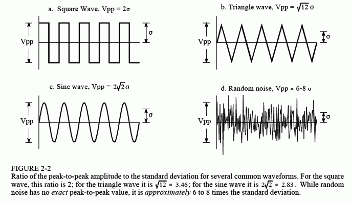
In the alternative notation: sigma = sqrt((x₀ -μ)² + (x₁ -μ)² + ... + (x_N-1 -μ)² / (N-1)). Notice that the average is carried out by dividing by N - 1 instead of N. This is a subtle feature of the equation that will be discussed in the next section. The term, σ², occurs frequently in statistics and is given the name variance. The standard deviation is a measure of how far the signal fluctuates from the mean. The variance represents the power of this fluctuation. Another term you should become familiar with is the rms (root-mean-square) value, frequently used in electronics. By definition, the standard deviation only measures the AC portion of a signal, while the rms value measures both the AC and DC components. If a signal has no DC component, its rms value is identical to its standard deviation. Figure 2-2 shows the relationship between the standard deviation and the peak-to-peak value of several common waveforms.

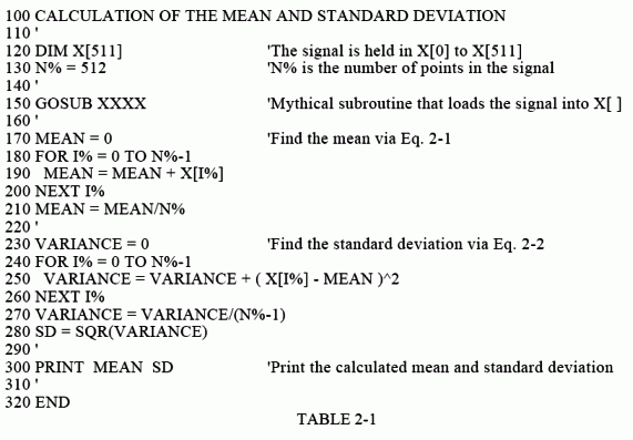
Table 2-1 lists a computer routine for calculating the mean and standard deviation using Eqs. 2-1 and 2-2. The programs in this book are intended to convey algorithms in the most straightforward way; all other factors are treated as secondary. Good programming techniques are disregarded if it makes the program logic more clear. For instance: a simplified version of BASIC is used, line numbers are included, the only control structure allowed is the FOR-NEXT loop, there are no I/O statements, etc. Think of these programs as an alternative way of understanding the equations used

in DSP. If you can't grasp one, maybe the other will help. In BASIC, the % character at the end of a variable name indicates it is an integer. All other variables are floating point. Chapter 4 discusses these variable types in detail.

This method of calculating the mean and standard deviation is adequate for many applications; however, it has two limitations. First, if the mean is much larger than the standard deviation, Eq. 2-2 involves subtracting two numbers that are very close in value. This can result in excessive round-off error in the calculations, a topic discussed in more detail in Chapter 4. Second, it is often desirable to recalculate the mean and standard deviation as new samples are acquired and added to the signal. We will call this type of calculation: running statistics. While the method of Eqs. 2-1 and 2-2 can be used for running statistics, it requires that all of the samples be involved in each new calculation. This is a very inefficient use of computational power and memory.

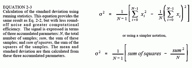
A solution to these problems can be found by manipulating Eqs. 2-1 and 2-2 to provide another equation for calculating the standard deviation:

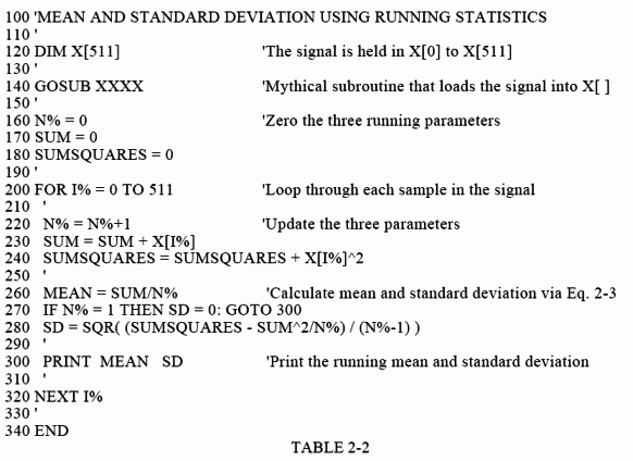
While moving through the signal, a running tally is kept of three parameters: (1) the number of samples already processed, (2) the sum of these samples, and (3) the sum of the squares of the samples (that is, square the value of each sample and add the result to the accumulated value). After any number of samples have been processed, the mean and standard deviation can be efficiently calculated using only the current value of the three parameters. Table 2-2 shows a program that reports the mean and standard deviation in this manner as each new sample is taken into account. This is the method used in hand calculators to find the statistics of a sequence of numbers. Every time you enter a number and press the Σ (summation) key, the three parameters are updated. The mean and standard deviation can then be found whenever desired, without having to recalculate the entire sequence.

Before ending this discussion on the mean and standard deviation, two other terms need to be mentioned. In some situations, the mean describes what is being measured, while the standard deviation represents noise and other interference. In these cases, the standard deviation is not important in itself, but only in comparison to the mean. This gives rise to the term: signal-to-noise ratio (SNR), which is equal to the mean divided by the standard deviation. Another term is also used, the coefficient of variation (CV). This is defined as the standard deviation divided by the mean, multiplied by 100 percent. For example, a signal (or other group of measure values) with a CV of 2%, has an SNR of 50. Better data means a higher value for the SNR and a lower value for the CV.