The Scientist and Engineer's Guide to
Digital Signal Processing
By Steven W. Smith, Ph.D.
Book Search
Table of contents
- 1: The Breadth and Depth of DSP
- 2: Statistics, Probability and Noise
- 3: ADC and DAC
- 4: DSP Software
- 5: Linear Systems
- 6: Convolution
- 7: Properties of Convolution
- 8: The Discrete Fourier Transform
- 9: Applications of the DFT
- 10: Fourier Transform Properties
- 11: Fourier Transform Pairs
- 12: The Fast Fourier Transform
- 13: Continuous Signal Processing
- 14: Introduction to Digital Filters
- 15: Moving Average Filters
- 16: Windowed-Sinc Filters
- 17: Custom Filters
- 18: FFT Convolution
- 19: Recursive Filters
- 20: Chebyshev Filters
- 21: Filter Comparison
- 22: Audio Processing
- 23: Image Formation & Display
- 24: Linear Image Processing
- 25: Special Imaging Techniques
- 26: Neural Networks (and more!)
- 27: Data Compression
- 28: Digital Signal Processors
- 29: Getting Started with DSPs
- 30: Complex Numbers
- 31: The Complex Fourier Transform
- 32: The Laplace Transform
- 33: The z-Transform
- 34: Explaining Benford's Law
How to order your own hardcover copy
Wouldn't you rather have a bound book instead of 640 loose pages?Your laser printer will thank you!
Order from Amazon.com.
Chapter 20: Chebyshev Filters
You must select four parameters to design a Chebyshev filter: (1) a high-pass or low-pass response, (2) the cutoff frequency, (3) the percent ripple in the passband, and (4) the number of poles. Just what is a pole? Here are two answers. If you don't like one, maybe the other will help:
Answer 1- The Laplace transform and z-transform are mathematical ways of breaking an impulse response into sinusoids and decaying exponentials. This is done by expressing the system's characteristics as one complex polynomial divided by another complex polynomial. The roots of the numerator are called zeros, while the roots of the denominator are called poles. Since poles and zeros can be complex numbers, it is common to say they have a "location" in the complex plane. Elaborate systems have more poles and zeros than simple ones. Recursive filters are designed by first selecting the location of the poles and zeros, and then finding the appropriate recursion coefficients (or analog components). For example, Butterworth filters have poles that lie on a circle in the complex plane, while in a Chebyshev filter they lie on an ellipse. This is the topic of Chapters 32 and 33.
Answer 2- Poles are containers filled with magic powder. The more poles in a filter, the better the filter works.

Kidding aside, the point is that you can use these filters very effectively without knowing the nasty mathematics behind them. Filter design is a specialty. In actual practice, more engineers, scientists and programmers think in terms of answer 2, than answer 1.
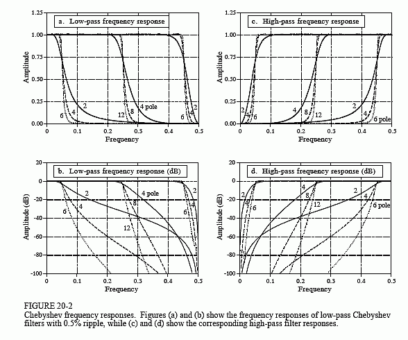
Figure 20-2 shows the frequency response of several Chebyshev filters with 0.5% ripple. For the method used here, the number of poles must be even. The cutoff frequency of each filter is measured where the amplitude crosses 0.707 (-3dB). Filters with a cutoff frequency near 0 or 0.5 have a sharper roll-off than filters in the center of the frequency range. For example, a two pole filter at fC = 0.05 has about the same roll-off as a four pole filter at fC = 0.25. This is fortunate; fewer poles can be used near 0 and 0.5 because of round-off noise. More about this later.
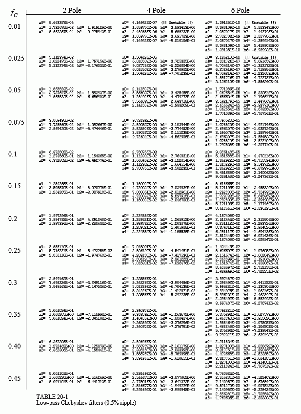
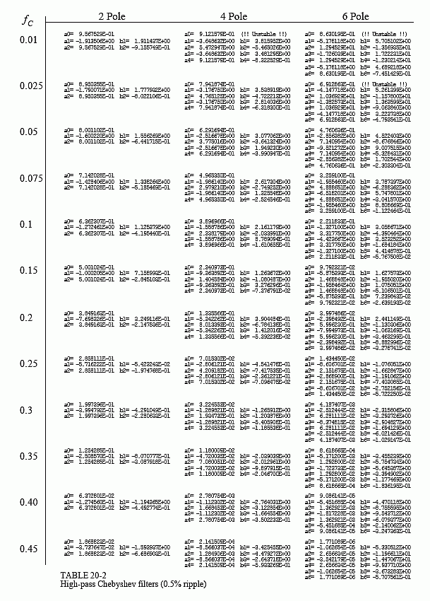
There are two ways of finding the recursion coefficients without using the z-transform. First, the cowards way: use a table. Tables 20-1 and 20-2 provide the recursion coefficients for low-pass and high-pass filters with 0.5% passband ripple. If you only need a quick and dirty design, copy the appropriate coefficients into your program, and you're done.


There are two problems with using tables to design digital filters. First, tables have a limited choice of parameters. For instance, Table 20-1 only provides 12 different cutoff frequencies, a maximum of 6 poles per filter, and no choice of passband ripple. Without the ability to select parameters from a continuous range of values, the filter design cannot be optimized. Second, the coefficients must be manually transferred from the table into the program. This is very time consuming and will discourage you from trying alternative values.
Instead of using tabulated values, consider including a subroutine in your program that calculates the coefficients. Such a program is shown in Table 20-4. The good news is that the program is relatively simple in structure. After the four filter parameters are entered, the program spits out the "a" and "b" coefficients in the arrays A[ ] and B[ ]. The bad news is that the program calls the subroutine in Table 20-5. At first glance this subroutine is really ugly. Don't despair; it isn't as bad as it seems! There is one simple branch in line 1120. Everything else in the subroutine is straightforward number crunching. Six variables enter the routine, five variables leave the routine, and fifteen temporary variables (plus indexes) are used within. Table 20-5 provides two sets of test data for debugging this subroutine. Chapter 31 discusses the operation of this program in detail.
