The Scientist and Engineer's Guide to
Digital Signal Processing
By Steven W. Smith, Ph.D.
Book Search
Table of contents
- 1: The Breadth and Depth of DSP
- 2: Statistics, Probability and Noise
- 3: ADC and DAC
- 4: DSP Software
- 5: Linear Systems
- 6: Convolution
- 7: Properties of Convolution
- 8: The Discrete Fourier Transform
- 9: Applications of the DFT
- 10: Fourier Transform Properties
- 11: Fourier Transform Pairs
- 12: The Fast Fourier Transform
- 13: Continuous Signal Processing
- 14: Introduction to Digital Filters
- 15: Moving Average Filters
- 16: Windowed-Sinc Filters
- 17: Custom Filters
- 18: FFT Convolution
- 19: Recursive Filters
- 20: Chebyshev Filters
- 21: Filter Comparison
- 22: Audio Processing
- 23: Image Formation & Display
- 24: Linear Image Processing
- 25: Special Imaging Techniques
- 26: Neural Networks (and more!)
- 27: Data Compression
- 28: Digital Signal Processors
- 29: Getting Started with DSPs
- 30: Complex Numbers
- 31: The Complex Fourier Transform
- 32: The Laplace Transform
- 33: The z-Transform
- 34: Explaining Benford's Law
How to order your own hardcover copy
Wouldn't you rather have a bound book instead of 640 loose pages?Your laser printer will thank you!
Order from Amazon.com.
Chapter 26: Neural Networks (and more!)
Chapters 19 and 20 show how to design recursive filters with the standard frequency responses: high-pass, low-pass, band-pass, etc. What if you need something custom? The answer is to design a recursive filter just as you would a neural network: start with a generic set of recursion coefficients, and use iteration to slowly mold them into what you want. This technique is important for two reasons. First, it allows custom recursive filters to be designed without having to hassle with the mathematics of the z-transform. Second, it shows that the ideas from conventional DSP and neural networks can be combined to form superb algorithms.
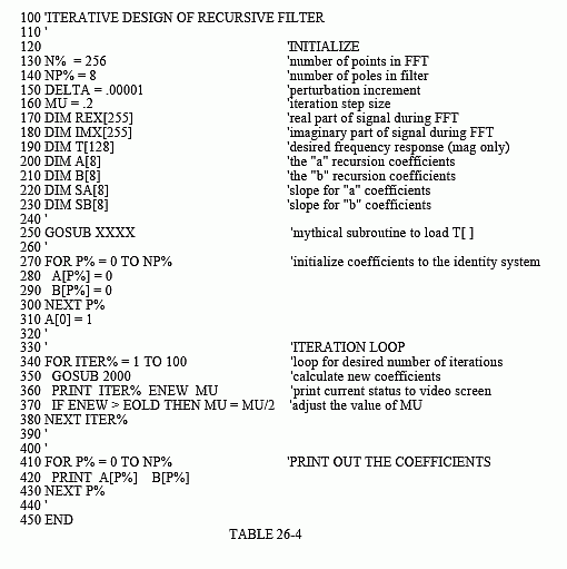
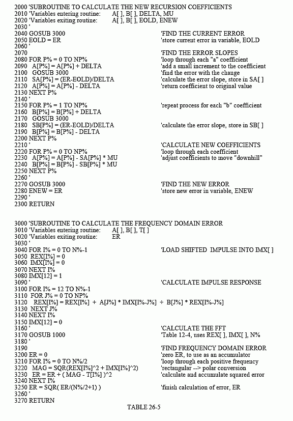
The main program for this method is shown in Table 26-4, with two subroutines in Table 26-5. The array, T[ ], holds the desired frequency response, some kind of curve that we have manually designed. Since this program is based around the FFT, the lengths of the signals must be a power of two. As written, this program uses an FFT length of 256, as defined by the variable, N%, in line 130. This means that T[0] to T[128] correspond to the frequencies between 0 and 0.5 of the sampling rate. Only the magnitude is contained in this array; the phase is not controlled in this design, and becomes whatever it becomes.
The recursion coefficients are set to their initial values in lines 270-310, typically selected to be the identity system. Don't use random numbers here, or the initial filter will be unstable. The recursion coefficients are held in the arrays, A[ ] and B[ ]. The variable, NP%, sets the number of poles in the designed filter. For example, if NP% is 5, the "a" coefficients run from A[0] to A[5], while the "b" coefficients run from B[1] to B[5].
As previously mentioned, the iterative procedure requires a single value that describes how well the current system is functioning. This is provided by the variable, ER (for error), and is calculated in subroutine 3000. Lines

3040 to 3080 load an impulse in the array, IMX[ ]. Next, lines 3100-3150 use this impulse as an input signal to the recursive filter defined by the current values of A[ ] and B[ ]. The output of this filter is thus the impulse response of the current system, and is stored in the array, REX[ ]. The system's frequency response is then found by taking the FFT of the impulse response, as shown in line 3170. Subroutine 1000 is the FFT program listed in Table 12-4 in Chapter 12. This FFT subroutine returns the frequency response in rectangular form, overwriting the arrays REX[ ] and IMX[ ].
Lines 3200-3250 then calculate ER, the mean squared error between the magnitude of the current frequency response, and the desired frequency response. Pay particular attention to how this error is found. The iterative action of this program optimizes this error, making the way it is defined very important. The FOR-NEXT loop runs through each frequency in the frequency response. For each frequency, line 3220 calculates the magnitude of the current frequency response from the rectangular data. In line 3230, the error at this frequency is found by subtracting the desired magnitude, T[ ], from the current magnitude, MAG. This error is then squared, and added to the accumulator variable, ER. After looping through each frequency, line 3250 completes the calculation to make ER the mean squared error of the entire frequency response.
Lines 340 to 380 control the iteration loop of the program. Subroutine 2000 is where the changes to the recursion coefficients are made. The first action in this subroutine is to determine the current value of ER, and store it in another variable, EOLD (lines 2040 & 2050). After the subroutine updates the coefficients, the value of ER is again determined, and assigned to the variable, ENEW (lines 2270 and 2280).
The variable, MU, controls the iteration step size, just as in the previous neural network program. An advanced feature is used in this program: an automated adjustment to the value of MU. This is the reason for having the two variables, EOLD and ENEW. When the program starts, MU is set to the relatively high value of 0.2 (line 160). This allows the convergence to proceed rapidly, but will limit how close the filter can come to an optimal solution. As the iterations proceed, points will be reached where no progress is being made, identified by ENEW being higher than EOLD. Each time this occurs, line 370 reduces the value of MU.
Subroutine 2000 updates the recursion coefficients according to the steepest decent method: calculate the slope for each coefficient, and then change the coefficient an amount proportional to its slope. Lines 2080-2130 calculate the slopes for the "a" coefficients, storing them in the array, SA[ ]. Likewise, lines 2150-2200 calculate the slopes for the "b" coefficients, storing them in the array, SB[ ]. Lines 2220-2250 then modify each of the recursion coefficients by an amount proportional to these slopes. In this program, the proportionality constant is simply the step size, MU. No error term is required in the proportionality constant because there is only one example to be matched: the desired frequency response.
The last issue is how the program calculates the slopes of the recursion coefficients. In the neural network example, an equation for the slope was derived. This procedure cannot be used here because it would require taking the derivative across the DFT. Instead, a brute force method is applied: actually change the recursion coefficient by a small increment, and then directly calculate the new value of ER. The slope is then found as the change in ER divided by the amount of the increment. Specifically, the current value of ER is found in lines 2040-2050, and stored in the variable, EOLD. The loop in lines 2080-2130 runs through each of the "a" coefficients. The first action inside this loop is to add a small increment, DELTA, to the recursion coefficient being worked on (line 2090). Subroutine 3000 is invoked in line 2100 to find the value of ER with the modified coefficient. Line 2110 then calculates the slope of this coefficient as: (ER - EOLD)/DELTA. Line 2120 then restores the modified coefficient by subtracting the value of DELTA.
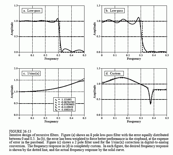
Figure 26-13 shows several examples of filters designed using this program. The dotted line is the desired frequency response, while the solid line is the


frequency response of the designed filter. Each of these filters requires several minutes to converge on a 100 MHz Pentium. Figure (a) is an 8 pole low-pass filter, where the error is equally weighted over the entire frequency spectrum (the program as written). Figure (b) is the same filter, except the error in the stopband is multiplied by eight when ER is being calculated. This forces the filter to have less stopband ripple, at the expense of greater ripple in the passband.
Figure (c) shows a 2 pole filter for: 1/sinc(x). As discussed in Chapter 3, this can be used to counteract the zeroth-order hold during digital-to-analog conversion (see Fig. 3-6). The error in this filter was only summed between 0 and 0.45, resulting in a better match over this range, at the expense of a worse match between 0.45 and 0.5. Lastly, (d) is a very irregular 6 pole frequency response that includes a sharp dip. To achieve convergence, the recursion coefficients were initially set to those of a notch filter.
