The Scientist and Engineer's Guide to
Digital Signal Processing
By Steven W. Smith, Ph.D.
Book Search

Table of contents
- 1: The Breadth and Depth of DSP
- 2: Statistics, Probability and Noise
- 3: ADC and DAC
- 4: DSP Software
- 5: Linear Systems
- 6: Convolution
- 7: Properties of Convolution
- 8: The Discrete Fourier Transform
- 9: Applications of the DFT
- 10: Fourier Transform Properties
- 11: Fourier Transform Pairs
- 12: The Fast Fourier Transform
- 13: Continuous Signal Processing
- 14: Introduction to Digital Filters
- 15: Moving Average Filters
- 16: Windowed-Sinc Filters
- 17: Custom Filters
- 18: FFT Convolution
- 19: Recursive Filters
- 20: Chebyshev Filters
- 21: Filter Comparison
- 22: Audio Processing
- 23: Image Formation & Display
- 24: Linear Image Processing
- 25: Special Imaging Techniques
- 26: Neural Networks (and more!)
- 27: Data Compression
- 28: Digital Signal Processors
- 29: Getting Started with DSPs
- 30: Complex Numbers
- 31: The Complex Fourier Transform
- 32: The Laplace Transform
- 33: The z-Transform
- 34: Explaining Benford's Law
How to order your own hardcover copy
Wouldn't you rather have a bound book instead of 640 loose pages?Your laser printer will thank you!
Order from Amazon.com.
Chapter 6: Convolution
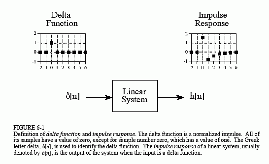
Let's summarize this way of understanding how a system changes an input signal into an output signal. First, the input signal can be decomposed into a set of impulses, each of which can be viewed as a scaled and shifted delta function. Second, the output resulting from each impulse is a scaled and shifted version of the impulse response. Third, the overall output signal can be found by adding these scaled and shifted impulse responses. In other words, if we know a system's impulse response, then we can calculate what the output will be for any possible input signal. This means we know everything about the system. There is nothing more that can be learned about a linear system's characteristics. (However, in later chapters we will show that this information can be represented in different forms).
The impulse response goes by a different name in some applications. If the system being considered is a filter, the impulse response is called the filter kernel, the convolution kernel, or simply, the kernel. In image processing, the impulse response is called the point spread function. While these terms are used in slightly different ways, they all mean the same thing, the signal produced by a system when the input is a delta function.
Convolution is a formal mathematical operation, just as multiplication, addition, and integration. Addition takes two numbers and produces a third number, while convolution takes two signals and produces a third signal. Convolution is used in the mathematics of many fields, such as probability and statistics. In linear systems, convolution is used to describe the relationship between three signals of interest: the input signal, the impulse response, and the output signal.
Figure 6-2 shows the notation when convolution is used with linear systems. An input signal, x[n], enters a linear system with an impulse response, h[n], resulting in an output signal, y[n]. In equation form: x[n] * h[n] = y[n]. Expressed in words, the input signal convolved with the impulse response is equal to the output signal. Just as addition is represented by the plus, +, and multiplication by the cross, ×, convolution is represented by the star, *. It is unfortunate that most programming languages also use the star to indicate multiplication. A star in a computer program means multiplication, while a star in an equation means convolution.
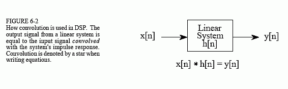
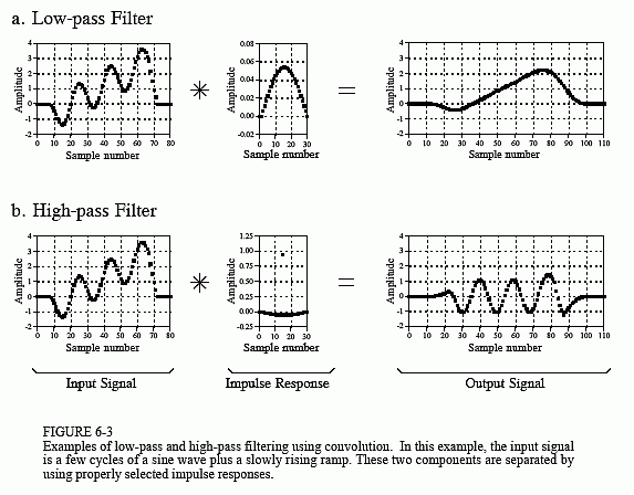
Figure 6-3 shows convolution being used for low-pass and high-pass filtering. The example input signal is the sum of two components: three cycles of a sine wave (representing a high frequency), plus a slowly rising ramp (composed of low frequencies). In (a), the impulse response for the low-pass filter is a smooth arch, resulting in only the slowly changing ramp waveform being passed to the output. Similarly, the high-pass filter, (b), allows only the more rapidly changing sinusoid to pass.
Figure 6-4 illustrates two additional examples of how convolution is used to process signals. The inverting attenuator, (a), flips the signal top-for-bottom, and reduces its amplitude. The discrete derivative (also called the first difference), shown in (b), results in an output signal related to the slope of the input signal.
Notice the lengths of the signals in Figs. 6-3 and 6-4. The input signals are 81 samples long, while each impulse response is composed of 31 samples. In most DSP applications, the input signal is hundreds, thousands, or even millions of samples in length. The impulse response is usually much shorter, say, a few points to a few hundred points. The mathematics behind convolution doesn't restrict how long these signals are. It does, however, specify the length of the output signal. The length of the output signal is
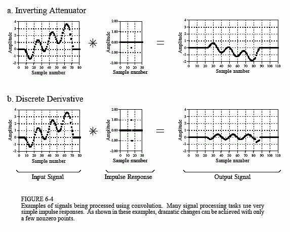
equal to the length of the input signal, plus the length of the impulse response, minus one. For the signals in Figs. 6-3 and 6-4, each output signal is: 81 + 31 - 1 = 111 samples long. The input signal runs from sample 0 to 80, the impulse response from sample 0 to 30, and the output signal from sample 0 to 110.
Now we come to the detailed mathematics of convolution. As used in Digital Signal Processing, convolution can be understood in two separate ways. The first looks at convolution from the viewpoint of the input signal. This involves analyzing how each sample in the input signal contributes to many points in the output signal. The second way looks at convolution from the viewpoint of the output signal. This examines how each sample in the output signal has received information from many points in the input signal.
Keep in mind that these two perspectives are different ways of thinking about the same mathematical operation. The first viewpoint is important because it provides a conceptual understanding of how convolution pertains to DSP. The second viewpoint describes the mathematics of convolution.
This typifies one of the most difficult tasks you will encounter in DSP: making your conceptual understanding fit with the jumble of mathematics used to communicate the ideas.